S-GIMME Tutorial
Parsons, J.T. & Johnson, A.D.
October 13, 2020
S-GIMME
Subgrouping GIMME was designed to enable researchers to identify clusters of individuals based only on their time-series data, with no a priori information regarding condition, behavior, or individual characteristics.
Specifically, S-GIMME conducts the community-detection algorithm Walktrap (Pons & Latapy, 2006) on temporal features available during GIMME model building. After arriving at the group-level effects, S-GIMME identifies effects that may be specific to each subgroup. Finally, as with the original GIMME algorithm, S-GIMME conducts individual-level searches. All weights are estimated at the individual level—even for those dynamic relations found to exist at the group or subgroup levels. Importantly, the researcher does not need to decide the number of subgroups – the algorithm finds the number. The final models contain reliable group-, subgroup-, and individual-level patterns that enable generalizable inferences, subgroups of individuals with shared model features, and individual-level patterns and estimates.
This document is a brief tutorial on using S-GIMME. Here we use a simulated time series data set available within gimme, simData. simData has 25 people with 200 time points and 10 variables (e.g., brain regions of interest or self report variables across time). The data were simulated so that the first 12 individuals have some paths in common (subgroup-level paths) and the second set of 13 individuals have some different paths in common. Hence there are 2 subgroups expected in the results, with different subgroup-level paths in addition to group-level paths (which everyone has estimated) and individual-level paths.
# Call the data from the gimme package into the environment
data("simData", package = "gimme")
To run S-GIMME, one calls the gimme (or equivalently, gimmeSEM) function with the field subgroup = TRUE. Other subgrouping options include sub_feature and sub_method.
# Run gimme using simData
gimme_output <- gimme(data        = simData,
                      subgroup    = TRUE,
                      sub_feature = "lag & contemp",
                      sub_method  = "Walktrap",
                      groupcutoff = .75,
                      subcutoff   = .51 )
data: indicate where the data are. When it is a list, you simply have to provide the name of the list object. If it is a directory where the data are stored, then you must provide header and sep arguments (see “Running GIMME” tutorial for details).
subgroup: must be TRUE (default is FALSE). This invokes the subgrouping algorithm.
sub_feature: option to indicate features to subgroup individuals. Default uses both “lag & contemp” relations; other options are to subgroup solely on similarities in “lagged” relations or “contemp” (contemporaneous) relations.
sub_method: option to change the community detection algorithm used to cluster individuals. Can use any approach that is in the igraph R package: “Walktrap” (default), “Infomap”, “Louvain”, “Edge Betweenness”, “Label Prop”, “Fast Greedy”, “Leading Eigen”, and “Spinglass”. S-GIMME has only been evaluated with Walktrap, which has been shown to be among the best algorithms for data with features seen in the GIMME algorithm (See this paper).
groupcutoff: the proportion of individuals for whom a path has to be significant for it to be added at the group level. This value should be more strict for large numbers of time points (i.e., high power to detect effects) and lower for smaller T or when the signal to noise ratio is thought to be small.
subgroupcutoff: defaults at .51, the proportion that has been tested the most in simulation studies. The same logic for groupcutoff follows here. A lower threshold than groupcutoff is typically used because, due to variable subgroup sizes, meeting the 75% threshold may be difficult (e.g., if only 7 people exist in a subgroup, that requires 6 of them to have the path).
Output
If subgroup = TRUE, a subgroup output directory is created with the following data:
- subgroupkPathCounts Contains counts of relations among lagged and contemporaneous variables for the kth subgroup.
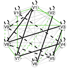
- subgroupkPlot (if plot = TRUE) Contains plot of group, subgroup, and individual level paths for the kth subgroup. Black represents group-level paths, grey represents individual-level paths, and green represents subgroup-level paths.
For example, the following two plots were produced in the output directory using simData.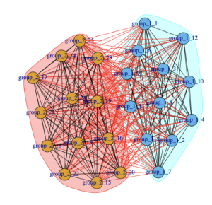
This is the summaryPathsplot (see Output tutorial for further explanation). Briefly, the green paths are paths that emerged for subgroups. Because two (or more) subgroups can theoretically have the same path be found as a subgroup-level path, the same color is used for all subgroup-level paths. Dashed lines indicate lagged relations, solid lines contemporaneous. Black lines are group-level and grey lines individual-level.
Note: if a subgroup of size n = 1 is discovered, subgroup-level output is not produced for that subgroup.
Evaluating Subgroups
Subgroups can be evaluated using the R package perturbR.
For example:
perturbRout <- perturbR(sym.matrix = gimme_output$sim_matrix,
                        plot       = TRUE,
                        resolution = 0.01,
                        reps       = 100,
                        errbars    = TRUE,
)
sym.matrix: the symmetric matrix that will be evaluated to see if community / subgroup solutions are robust. In gimme, this is the similarity matrix.
plot: logical indicating if plots should be made.
resolution: the resolution to use for the percent perturbed (alpha); .01 (the default) indicates that perturbations or rewiring of the network will occur in 1% increments. Larger values run faster.
reps: the number of repetitions to do at each level of perturbation. Lower values run faster.
Two plots are generated: “Comparison of original result against perturbed graphs: ARI” and “Comparison of original result against perturbed graphs: VI”. “ARI” is the adjusted Rand Index, where higher values indicate greater similarity between two cluster assignments (i.e., what subgroup each person is in). “VI” is Variation of Information, where lower values indicate greater similarity.
The ARI caps out at 1, so the upper bound is known. This is not true for the VI. So, results from completely random matrices with the same qualities as the matrix provided by the researcher (gimme_output$sim_matrix here) are compared. They provide the upper bound (red diamonds).
Below are the plots obtained from the results from simData’s similarity matrix.
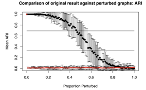
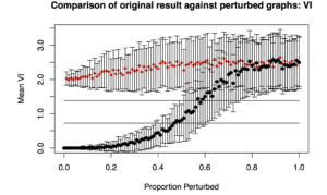
Essentially, what one is looking for is that it takes a long time for the ARI (top plot) to decrease given increased perturbations along the X axis. We similarly want it to take a while for the VI to increase. The idea is that for a robust solution, minor perturbations (or small proportion of edges rewired) should not drastically change the cluster solution or subgroups assignments.
See the perturbR vignette for more details on probing the output.
Additionally, the subgroups can be visually evaluated in a correlogram using corrplot.
For example:
a = cor(gimme_output$sim_matrix)
corrplot(a, method = "color")
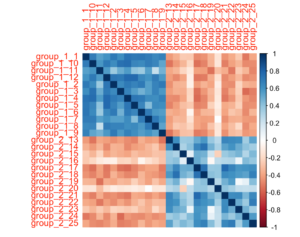
Note that the similarity matrix used here is already ordered based on the subgroup they are in.