Cara Arizmendi
2019-02-20
This vignette will cover basic functionality of ms-gimme including how to run ms-gimme, how to avoid potential problems when using ms-gimme, and how to use the solution.tree() function to explore the branching of multiple solutions.
Ms-gimme is a modification of gimme (group iterative multiple model estimation), allowing for the recovery of multiple uSEM (unified SEM) solutions with a data driven approach (Beltz and Molenaar, 2016).
Selecting multiple solutions gimme
To begin, we load a fitted gimme object, with which multiple solutions were found. This object is available as part of the gimme package and can be accessed as shown below.
library(gimme)
data(ms.fit, package="gimme")
Here we show the syntax used to arrive at the fitted object. To return multiple solutions, ms_allow should be TRUE. We only show the most relevant arguments to ms-gimme. We recommend that the default ar=FALSE be kept, as multiple solutions are unlikely to be found when ar=TRUE. Additionally, the default of subgroup=FALSE should be kept, as ms-gimme does not have the functionality for subgrouping. The remaining arguments are up to user discretion. For general gimme usage, we recommend standardize=TRUE; however, this is not the default since standardize=TRUE modifies the data. We do not recommend that ms_tol be greater than the default, but smaller tolerances can be set.
ms.fit <- gimme(data        = ms.sim,
                out         = '~/outputfolder/',
                ar          = FALSE,
                subgroup    = FALSE,
                standardize = TRUE,
                ms_allow    = TRUE,
                ms_tol      = 1e-5)
Exploring output object
Tree table
The function solution.tree() allows for exploration of diverging solutions. Below, we see that there were six different solutions at the group level. The first branch occured at ‘V1~V3’ versus ‘V3~V1.’ Within the solution where ‘V1~V3’ was selected, another divergence occurs between ‘V2~V4’ and ‘V4~V2.’
solution.tree(ms.fit, level = "group", cols="stage")
#>                               levelName stage
#> 1  NULL MODEL
#> 2   ¦--V1~V3
#> 3   ¦   ¦--V2~V4
#> 4   ¦   ¦   °--V3~V2
#> 5   ¦   ¦       °--V4~V1lag
#> 6   ¦   ¦           °--V3~V3lag
#> 7   ¦   ¦               °--V4~V4lag     group
#> 8   ¦   °--V4~V2
#> 9   ¦       ¦--V2~V3
#> 10  ¦       ¦   °--V3~V3lag
#> 11  ¦       ¦       °--V4~V3lag         group
#> 12  ¦       °--V3~V2
#> 13  ¦           °--V2~V4lag
#> 14  ¦               °--V4~V4lag
#> 15  ¦                   °--V3~V3lag     group
#> 16  °--V3~V1
#> 17      ¦--V2~V4
#> 18      ¦   °--V4~V3
#>gt; 19      ¦       °--V4~V2
#> 20      ¦           °--V1~V3lag
#> 21      ¦               °--V3~V3lag
#> 22      ¦                   °--V2~V3lag group
#> 23      °--V4~V2
#> 24          °--V2~V3
#> 25              °--V1~V3lag
#> 26                  °--V4~V1lag
#> 27                      ¦--V1~V3        group
#> 28                      °--V3~V3lag     group
Tree plot
We can also produce a plot version of the above table.
solution.tree(ms.fit, level = "group", plot.tree = TRUE)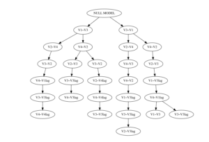
Deciding between models
We refer users to Beltz and Molenaar (2016) for guidance on model selection. The AIC is the most widely used fit statistic for model selection and can be accessed in the gimme object as partially shown below or in file ‘summaryFit.csv’ in the output folder if an output folder is specified.
ms.fit$tables$summaryFit[1:10,]
#>                          subj grp_sol ind_sol   chisq df npar pvalue
#> fit_info_lav    A1_Phi1_subj1       1       1 11.2634 16   28 0.7929
#> fit_info_lav1   A2_Phi1_subj2       1       1  8.9444 16   28 0.9157
#> fit_info_lav2   A3_Phi1_subj3       1       1 10.8864 16   28 0.8164
#> fit_info_lav3   A4_Phi1_subj4       1       1 27.1169 16   28 0.0402
#> fit_info_lav4   A5_Phi1_subj5       1       1  8.1448 16   28 0.9444
#> fit_info_lav5   A6_Phi1_subj6       1       1 14.8355 16   28 0.5367
#> fit_info_lav6   A7_Phi1_subj7       1       1  8.5935 16   28 0.9292
#> fit_info_lav7   A8_Phi1_subj8       1       1 21.0296 16   28 0.1774
#> fit_info_lav8   A9_Phi1_subj9       1       1 15.6445 16   28 0.4780
#> fit_info_lav9 A10_Phi1_subj10       1       1 19.5190 16   28 0.2427
#>                rmsea   srmr   nnfi    cfi      bic      aic      logl
#> fit_info_lav  0.0000 0.0250 1.0093 1.0000 1460.856 1388.193 -666.0963
#> fit_info_lav1 0.0000 0.0192 1.0145 1.0000 1502.374 1429.711 -686.8554
#> fit_info_lav2 0.0000 0.0189 1.0115 1.0000 1572.892 1500.228 -722.1141
#> fit_info_lav3 0.0838 0.0521 0.9522 0.9727 1962.509 1889.846 -916.9230
#> fit_info_lav4 0.0000 0.0263 1.0222 1.0000 1731.804 1659.141 -801.5703
#> fit_info_lav5 0.0000 0.0385 1.0032 1.0000 1723.683 1651.020 -797.5099
#> fit_info_lav6 0.0000 0.0278 1.0166 1.0000 1570.380 1497.716 -720.8582
#> fit_info_lav7 0.0563 0.0335 0.9827 0.9901 1852.670 1780.007 -862.0035
#> fit_info_lav8 0.0000 0.0342 1.0013 1.0000 1860.983 1788.320 -866.1600
#> fit_info_lav9 0.0471 0.0289 0.9916 0.9952 1605.973 1533.310 -738.6548
#>                           status checkPsi
#> fit_info_lav  converged normally    FALSE
#> fit_info_lav1 converged normally    FALSE
#> fit_info_lav2 converged normally    FALSE
#> fit_info_lav3 converged normally    FALSE
#> fit_info_lav4 converged normally    FALSE
#> fit_info_lav5 converged normally    FALSE
#> fit_info_lav6 converged normally    FALSE
#> fit_info_lav7 converged normally    FALSE
#> fit_info_lav8 converged normally    FALSE
#> fit_info_lav9 converged normally    FALSE
Reference
Adriene M. Beltz & Peter C. M. Molenaar (2016) Dealing with Multiple Solutions in Structural Vector Autoregressive Models, Multivariate Behavioral Research, 51:2-3, 357-373, DOI: 10.1080/00273171.2016.1151333