Written by Nat Heddaeus, James Thompson, and Rujula Yete
Observations
In this project, we used radio astronomy to observe pulsars. These are neutron stars that emit radiation pulses with each rotation. We specifically analyzed the PSR 0329+54 pulsar, located about 3,460 lightyears away in the Camelopardalis constellation. We used the telescope at the Green Bank Observatory. The frequency for the observation was 1395 MHz with a duration of 180 seconds and an integration time of 0.021 seconds.
PSR 0329+51 Analysis
Initial Light Curve
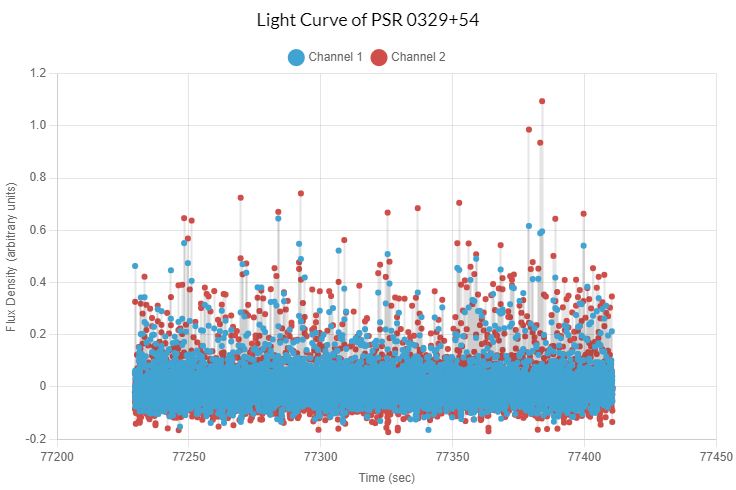
Our first analysis step was to upload the data from the telescope into the Skynet plotting tool. We can then see an initial light curve, showing the signals detected by the two channels. From this plot, we can hear an initial sonification, as well as estimate the period (time between the pulses). Since we saw consistent spikes around every 0.7 seconds, we adjusted the background scale value to 0.8 in order to visualize this estimate on the light curve. Then, we used this estimate to adjust the periodogram.
Periodogram
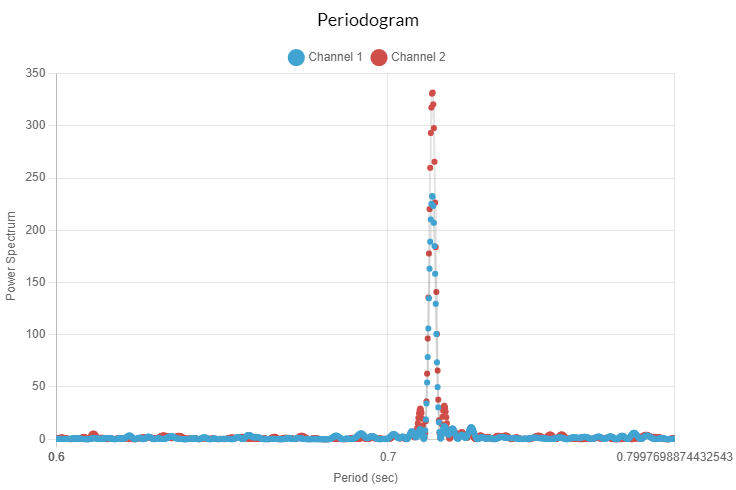
The periodogram graphs the various periodicities, or the amount of data that follows each period. As we expected, the highest spike was around 0.7, further indicating that this is near the actual period of the pulsar. There was also a significant spike around 0.35, since this is the half value of 0.7. Since we knew that the period was around 0.7, we could adjust the start and stop values to contain 0.7, such as starting at 0.6 and stopping at 0.8. We also used the algorithm with 1000 data points, since the spike was apparent with this amount of data. By looking at the data points on the graph, we can narrow this range even more, finding that the spike is precisely at 0.7146.
Folded Light Curve
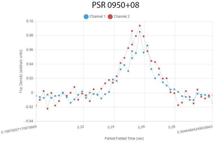
Now that we’ve pinpointed the period of our data, we can emphasize the signal by overlaying all the periods of our data: this way, the peaks of the graph all line up and so the combination is more apparent. To ensure that our period is right, we can try varying it slightly: if the period we obtained results in the largest spikes, we can be confident it’s correct.
Sonogram
Another way of representing our data is through sound: we can create an audio file from our data, letting the intensity of the graph correspond to the volume of the sound. Sometimes this makes it possible to hear the period of the pulsar as a faint beat in the audio file even if it’s not apparent visually. After making the folded light curve, we can also sonify this to get a clearer version of our signal
Calibration of Second Polarization Channel to First Via Unpolarized Source
From basic physics, we know that light consists of electromagnetic waves. We’re familiar with the fact that any given beam of light is traveling in a specific direction, but what’s less familiar is the fact that the underlying wave is also oscillating in some particular direction perpendicular to this. For instance, an electromagnetic wave traveling right at you could be oscillating up and down, left and right, or somewhere in between. This is called the light’s polarization.
Now, it turns out that whether the light we’re seeing from the neutron star is polarized gives us clues about the light’s origin. One familiar source of light is thermal emission, or emission due to an object’s temperature: it’s the reason why people are visible on infrared cameras. Importantly, thermal emission is always unpolarized. However, other types of emission result in polarized light: in particular, some kinds of emission resulting from magnetic fields yield polarized light.
The intensity data we receive from our neutron star comes in two channels detecting light of two different, perpendicular polarizations. However, initially the data are not expressed in physical units; although the data from one channel is internally meaningful, we can’t compare the two. Before we can determine whether the light from our star is polarized, we need to calibrate our channels (you might wonder why the observatory hasn’t already done this; the answer is that the internal electronics of the two channels drift over time, so any given calibration isn’t useful for very long).
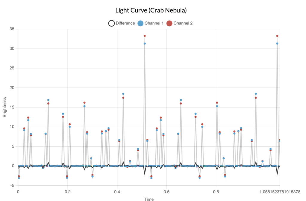
To do this, we collected data at about the same time from a roughly unpolarized source, the Crab Nebula. When we look at the data from this source, we know the two channels should be in agreement, and we can find the factor we need to scale them by to make this happen:
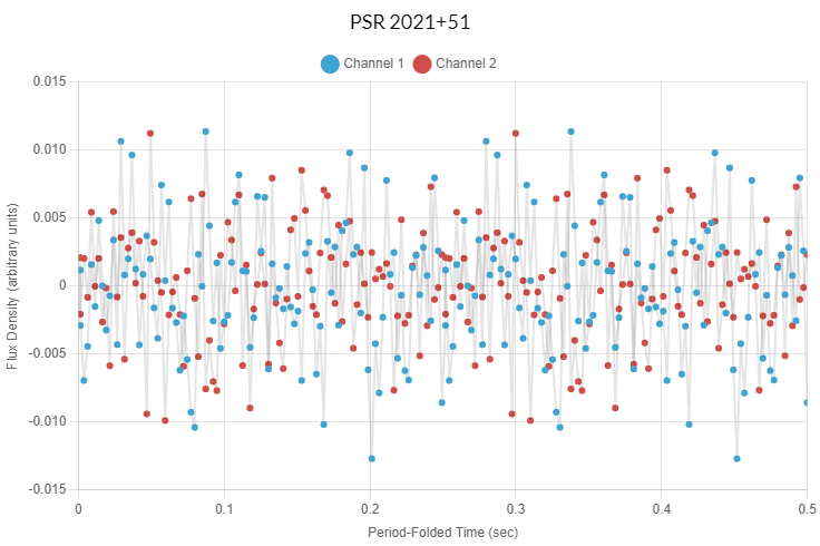
We can then transfer this factor over to our other data so that the relative values between the channels are meaningful. When we do so, we find that the difference between the two channels varies significantly over time:
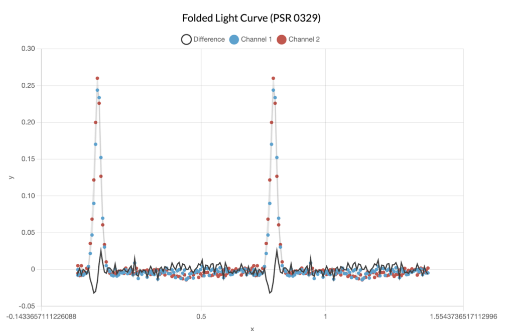
This is not what we would expect from an unpolarized source, so there must be a different emission mechanism. Our results turn out to line up very well with the existing model of pulsar emissions called the lighthouse model.
We’re all familiar with the Earth’s magnetic field. Pulsars also have magnetic fields, but they’re much stronger than those of Earth. Though the exact reason is not known, it seems that where pulsars’ magnetic field lines interact with the surface of the star, they ionize nearby particles. As dictated by Maxwell’s Equations, these charged particles then spiral out around the magnetic field lines of the star. These magnetic field lines are curved, and so in the course of following them, the charged particles have to change their orientation. In doing so, by basic electromagnetism, they emit light. Moreover, this light is polarized due to the orientation of the field lines.
Now, as the star rotates, the direction the light is emitted in changes: thus, a beam of light originating at the pulsar sweeps across the sky. When it hits Earth, the pulsar appears to be on. When it doesn’t, the pulsar is off. Moreover, as the beam of light changes direction, we expect the polarization of the received light to change, which is exactly what we observed above.
Additional Folded Light Curves and Sonograms
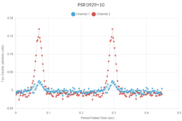
PSR 0929+10 Velocity and Size
Through our plots, we found the period of PSR 0929+10 to be 0.2265 seconds. Using the bounds D < cP/𝜋, we calculate the upper bounds of the diameter of PSR 0929+10 to be less than 21629.1568 km or 0.000002622 earth diameters.
Sonograms for High Velocity Pulsars
Below are three pulsars of increasing velocities, including the fastest known pulsar, PSR J1748-2446ad.
Updated Bounds
The rotation period of PSR J1748-2446ad is known to be 0.0013959548 seconds. Using the bounds D <cP/𝜋, we calculate the upper bounds of the diameter of PSR J1748-2446ad to be less than 133.3039 km, or 1.6157×10^-8 earth diameters.