Stars are some of the brightest, most beautiful, and complex entities that encompass our vast cosmos. The life cycle of a star is that of an intricate, transformational, and extensive process. The various processes of changes that a star goes through in its magnanimous life is known as stellar evolution. In this module, we will look at three distinct star clusters and process, analyze, and compare them to uncover key properties about the clusters such as age, color, luminosity, and temperature.
(Written by: Saki Male)
Young Section—IC 2948
Youngest goes first! The star cluster I chose to observe was IC 2948. This one stood out to me because of its background dust and particularly bright stars. Of course, I just couldn’t help but use one of Skynet’s CTIO’s telescopes, PROMPT-6, for its impressively little amount of atmospheric blurring. I used four filters, R for red (35.43s), V for green (47.24s), B for blue (70.87s), and I for near-infrared (35.43s). The I filter would not be used in the final image, but rather to be more helpful in creating an accurate HR diagram later on. Each of these filters would be repeated 5 times each, with 30 minutes between each set to combat any possible ghosts from previous observations (and to give everybody in the class the opportunity to get some data). Unfortunately, my observation only returned 4 of the 5 V filter images because of a small issue at CTIO, which gave me some issues I will discuss momentarily. After placing the observation during a decent time (dark moon cycle), I just had to wait!
After getting the images back, they were looking pretty good! Of course, as per usual with PROMPT-6, I had to clean up the bad column using a special advanced string operation made for the telescope. Next, I aligned the images, which was easy since there were enough stars in the image to use the World Coordinate System (WCS) for aligning. Stacking the images was where I faced some trouble. A new approach to stacking was used in order to combat the normal “hot pixels” that would appear without using any form of rejection/cleaning. By using “chauvenet” rejection with Low and High values of 1 (to reject high and low outliers), I was able to remove hot pixels from my stacks altogether. I used PROMPT-6 for all my images, so I had scaling set to “none” (didn’t need to account for different telescopes). This is where I encountered an issue that stumped my progress for a while. In my final image, the hot pixels from the green (V) stack remained. Not only did it make my image a little ugly, it was throwing off my color values as well I believe. After speaking with Dan Reichart, I was recommended to try the stacks again using “rcr” as the rejection mode, over chauvenet, which wouldn’t have a problem with the fact that I had 4 V filter images instead of 5. Thanks to his wisdom (lol), I ended up with a stunning start for a final image, absent of any apparent defects!
Coloring the image was quite easy after having some practice with it from a previous project. I used the Histogram color balancing mode, collecting zero points for each layer to get accurate colors! After syncing the layers to the B filter stack, since the blue stars were absolutely the brightest in the image, the image was looking incredible. The final touch was adjusting the color values based on any possible E(B-V) reddening in the image. This value to account for (0.37) was found through my creation of an HR diagram, which we will look at shortly. But first let’s take a look at that incredible young star cluster.
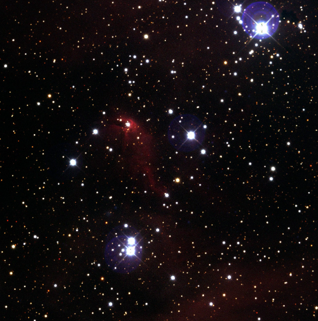
Figure 1 – Young Cluster
Next, I began the process of creating a Hertzsprung-Russell (HR) diagram to learn more about the cluster’s age, metallicity, reddening, and more. I used Afterglow’s source extraction to photometer all the stars possible in the Red layer since it’s the most likely to see the dimmer stars that appear more red. My browser was crying… Then I used the photometry tab to measure the brightness of all my sources. My browser just finished dying a little, then after doing so, I used batch photometry to copy those values for the other layers as well. After opening Skynet’s plotting software, I was able to begin building the HR diagram! I started by selecting the “Cluster Pro Plus” option (since we’re doing some serious stuff) and uploading my giant batch photometry CSV file. As you’ll see below, Cluster Pro Plus allowed me to plot two diagrams at the same time. For context, the x-axis represents the stars’ intrinsic colors (redder→lower magnitude & cooler, bluer→higher magnitude & hotter). The y-axis represents the absolute magnitude.
* For the first diagram (Skynet Blue), I used B – R data on the x-axis & V data on the y-axis.
* For the second (Skynet Red), I used V – I data on the x-axis & R data on the y-axis.
I decreased the data retrieval radius of stars in the image to focus on the stars that are actually in the cluster, which cut out field stars. This made it a bit easier to see the star cluster I was actually working with instead of being full of other stars that just happen to be in the image. Then, I began to play with the age, metallicity, distance, and reddening sliders until the black line (what the HR diagram should look like at those settings) matched with my stars! This took a bit to get used to, and it’ll never be perfect, but I think it’s pretty decent! As we can see, this cluster is truly (relative to other star clusters) a young one!
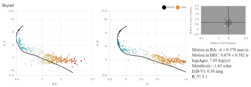
Figure 2
This is great, but it could be better! So, I added in archival data using Gaia and 2MASS. For these, the plotting would be a little different, but would improve the plot. Since there are a LOT of stars now, compared to just my Skynet data, I used “Lock Cuts” to permanently remove the field stars I already removed from the data, which sped things up on the browser significantly.
* For the first diagram (Gaia), I used BP – RP for the x-axis & G for the y-axis.
* For the second diagram (2MASS), I used J – K for the x-axis & H for the y-axis.
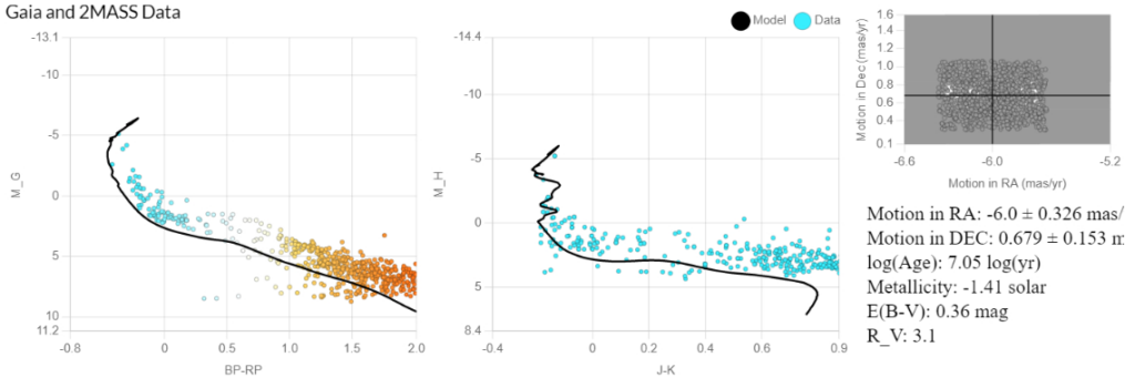
Figure 3
(Written by: Nathan Flinchum)
Intermediate Section—NGC 4349
Next up, we have an intermediate star cluster known as the NGC 4349. Now, you might be wondering: What’s the difference between young star clusters and intermediate star clusters? Well, the answer primarily pertains to the cluster’s age. As the intermediate star clusters are a little bit more progressed in their years than the young, we tend to see a higher metallicity and a lower reddening effect. Just to summarize again, metallicity in star clusters is proportional to the fragment of heavier elements (metals), and reddening is the process in which the interstellar medium (gas and dust) that collects around the star affects short and long wavelength radiations to different extents. Ultimately, reddening results in stars appearing redder than they actually are—further robbing distant stars of their blue-ish color.
But, let’s not get too ahead of ourselves—we have to explain how we even came to our final product of the NGC 4349 star cluster! So, for this observation, we utilized the PROMPT-6 telescope located in Cerro Tololo Inter-American Observatory in Chile. For this observation, we opted to use the filters B, V, and R, as they would be best in attempting to capture the natural colors that are seen with the human eye. Also, we used filter I to have a redder coverage to better differentiate the star cluster’s characteristics in the observation such as its metallicity and age. The observation had a total of 20 exposures taken, with each filter having 5 exposures. The exposure length for each image in the B filter was 62.99 seconds, the V filter was 27.56 seconds, the R filter was 15.75 seconds, and the I filter was 19.69 seconds. Also, the field of vision (FOV) for PROMPT-6 is approximately 14.8 x 15.1 arcmins with a pixel size of 2017 x 2051 pixels.
Just like with the young star cluster, IC 2948, the process was similar in the aligning, stacking, and color calibration. Prior to stacking, we were able to isolate the bad pixels and correct them using a specific pixel operation string that is plugged into our program known as Afterglow. Once we corrected the bad columns, we were able to align all of the 20 exposures in the observation and proceeded to stack the 5 exposures for each filter using the ‘Chauvenet’ rejection. The Chauvenet rejection helps to clarify the background of exposures with the removal of bad pixels. Next, after grouping all of the stacks into a single file, turning off the I filter stack, coloring the B stack blue, then the V stack green, and the R stack red, I was able to use aperture photometry to measure the brightness of each stack. After the process of using photometry and extracting sources to make thousands of measurements, we received the NGC 4349 batch photometry data.
You may be asking yourself: What’s next? Well, just like with the young star cluster, IC 2948, we uploaded our batch photometry data into OPIS!/MWU! graphing tool and began the construction of the H-R diagrams. Before I go into anymore depth, I want to reiterate what the H-R diagrams mean: on the x-axis we plot the star’s magnitude which comes across as its intrinsic color (the blue depicts the magnitude of the short-wavelength and the red depicts the long-wavelength), and the y-axis scales the absolute colors of the star cluster. So, for the first H-R diagram we used the filters (and in this order) B, R, V and then for the second diagram, we used the filters V, I, R. After using the tools ‘Motion in Ra’ and ‘Motion in Dec’ to eliminate field stars on the diagrams, I changed the E(B-V) to 0.3 mag to help correct the dust that also dims the star’s light, and decreased the distance to 1.61. Then, we increased the age to 8.61 log(yr) and moved the metallicity to 0.02 solar. At this star cluster’s age, we see a lot of main sequence stars which have hydrogen-burning cores.
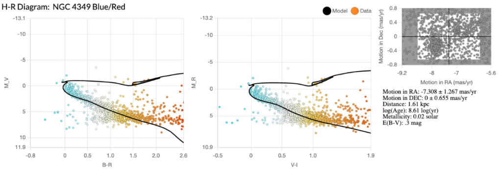
Figure 4
In the H-R diagram for the B and R filters above, I prioritized shaping my isochrone to the curve of my data (which dealt with the measure of the metallicity). Also, increasing the E(B-V) allowed my data to align more with the isochrone along the bottom line while getting the isochrone to touch the red giants along the top line (above the 0 mark on the y-axis). Unfortunately, I did have trouble trying to get the isochrone to ride below the range of binaries on the main sequence along with getting the isochrone to touch the data towards the end of the sequence on the right of the diagram.
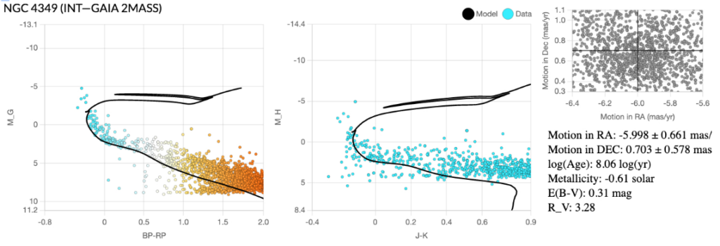
Figure 5
In the H-R diagram above, it is a combination of the data from NGC 4349 and the archival data from ‘Gaia’ and ‘2Mass’. Just to reiterate, Gaia is a telescope located in space and helps to model the faint end of the cluster. Gaia utilizes three filters: BP, G, and RP. Then, 2Mass is a near-infrared survey that is composed of two telescopes on Earth. 2Mass utilizes three filters: J, H, and K. With these filters, the issue of dust interfering with coloring and brightness is less apparent.
So, how did I go about configuring the H-R diagram with Gaia and 2Mass? Basically, it’s the first diagram but then add the step of turning on the ‘Lock Cuts’ button to permanently remove the field stars, and select the ‘Gaia’ and ‘2Mass’ while also selecting ‘Fetch Data’. Now, I didn’t deviate too far from the first H-R diagram with the original measurements—I lowered the age to 8.06 log (yr), decreased the metallicity to -0.61 solar, and increased the E(B-V) to .31 mag.
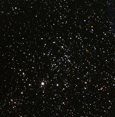
Figure 6 – Intermediate Cluster
After processing the dust and the reddening of the NGC 4349 data, I was able to go back into Afterglow to help emphasize the intrinsic colors of the star cluster. All that was done in this step was to try to re-calibrate the colors using the E(B-V) value collected from the process with the H-R diagrams.
(Written by: Delanie Mitchell)
Old Section—NGC 3201
Finally we arrive at the old star cluster. I chose NGC 3201 as my old globular cluster, and then went to Skynet to place the observation. For the telescope, just like the other star clusters we observed, I utilized Prompt 6 in Cerro Tololo Interamerican Observatory. For the filters I used B, V, and R, which are good at modeling what the human eye sees naturally, as well as the I filter, which is helpful in modeling the star clusters age and metallicity. On the exposures page, I ensured that each filter had 5 exposures for a grand total of 20. Each filter required its own individual exposure duration, with B being 70.87 seconds, V being 59.06 seconds, R being 47.24 seconds, and I being 23.62 seconds. I also made sure to repeat these sets of exposures five times with a 30-minute delay between each exposure set.
Once the images came back from Skynet, we first had to clean, align, and stack the images before we could begin any color processing. Once I uploaded my images to Afterglow and ensured there weren’t any problems, I went ahead to the cleaning stage. To do this I went to the “show pixel operations” tab, selected advanced, selected the images under “additional images,” and inputted a long pixel operation string that would overwrite the existing files. This was done in order to remove the bad columns present in the images, a feature commonly found in the Prompt 6 telescope, remove bad pixels, and just clean up the images as a whole. Once this simple task was done, I moved on to the aligning stage. To align the images, we used the WCS (world coordinate system), which matches pixel coordinates of the image’s stars to the known RA/Dec coordinates of catalog stars and aligns them to each other. On the aligner tab, I selected all of the images across the filters, selected a reference image, enabled Crop, Rotation, Scale, and Skew, set the mode to WCS (making sure that mosaic mode was disabled and the WCS grid point value was 100), and submitted the job. After successfully aligning my images, I moved on to the stacking. In the stacker tab, I selected all of the images for one filter, set the rejection mode to “chauvenet” with both low and high settings being set to 1, set the scaling to average and the smart stacking to SNR, and enabled propagate mask. I then submitted the job and repeated the process for the other three filters until I had all my B, V, R, and I stacks completed.
After these crucial initial steps of cleaning, aligning, and stacking, we can move on to color calibration. To start, I grouped all of the stacks together, colored the stacks, with B being blue, V being green, and R being red, and clicked the eye icon to hide the I stack. Next it was time to color balance the stacks by using the brightnesses of background stars. To do this I first viewed the color combined image and changed the color balance mode from “percentile” to “histogram fitting” under the display settings. Then I selected the photometric color calibration tool in order to measure the zero points, left the extinction at 0 (which makes the stars appear as they do from Earth), and ensured that “Blackbody Peaking in B Appears White” was selected, and then pressed the “calibrate colors” button. Before color balancing, however, it’s necessary to select a layer to sync the brightness and contrast levels to. For my old cluster, the brightest star was white, therefore I used the V or green layer as my reference layer. I then changed the stretch mode to Midtone, pressed the default target setting, and adjusted the background level until it was just below the curve on the histogram.
Once we color balanced the image, it was time to utilize aperture photometry to measure the brightness of each star in each of the stacks. In order to do this I had to go to the “Photometry Calibration” tab, enable “use catalog to calibrate zero point offset,” and select the APASS catalog. I clicked on the red stack, as this is the stack with the best detected sources. Then I went to the Source Catalog tab and enabled “include sources from other files,” Source Markers, and Centroid Clicks, and pressed +Add Sources and Source Extraction. I made sure to select all four of my stacks and batch photometered the images. After this was all done, I was left with a downloadable file of my “batch photometry data.”
With my batch photometry data, it was now time to assemble the HR diagrams. We went to the OPIS!/MWU! graphing tool and clicked on “Cluster Pro Plus” which pulled up two HR diagrams. I then opened my data and plotted B, R, and V on the first HR diagram and plotted V, I, and R on the second. In the graph tool that displayed the proper motions of the cluster stars I used the “Motion in RA” and “Motion in Dec” sliders in order to crop out field stars, allowing for a less chaotic looking HR diagram. I then turned to the sliders and adjusted each one in order to best fit. Since this is an old globular cluster, I automatically moved the age slider to its maximum setting at 10.2 log(yR). I set my E(B-V), the amount of dust we need to correct for, to 0.19 mag, and set the metallicity, aka how much of everything except hydrogen and helium was in the gas where cluster stars formed, to -1.4 solar.
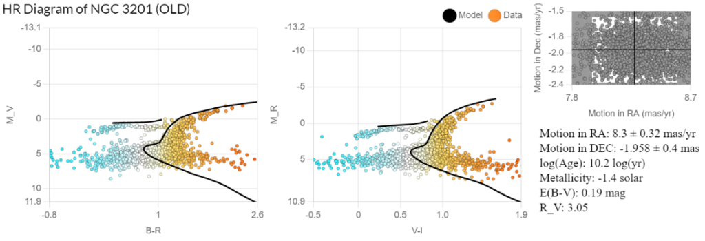
Figure 7
Above you can see the completed HR diagram with the aforementioned values. When creating the diagram, I tried my best to match the isochrone to the horizontal branch stars as it’s much easier to match the isochrone to those then it is to match it to the precise turn off point. The stars on the right appear to be in a sort of C shape, and so the isochrone touches the top of the data and begins to tear off near the bottom.
When the first round of HR diagrams were finally completed, it was time to refine our measurements and add in archival data from Gaia and 2MASS. At this point, we didn’t need to collect any more data, all we had to do was manipulate the original HR diagram. To do this I first changed the filters to BP (blue), G (green), and RP (red) for Gaia and J (bluer), H, and K (redder) for 2MASS. Then I pressed the “Lock Cuts” button to remove field stars that had already been cropped out, selected GAIA and 2MASS at the bottom of the diagrams, and pressed “Fetch Data.” After this finished running, I adjusted the age, metallicity and the reddening (E(B-V)) ever so slightly to fit the isochrone to the data.
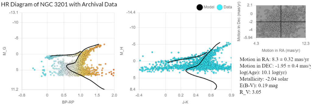
Figure 8
Above is the HR diagram of the old globular cluster with the addition of the archival data from Gaia and 2MASS. I once again tried to make sure that the isochrone matched the horizontal branch stars and I think I achieved that goal. Again, you can see the stars don’t follow the isochrone near the bottom right, however the isochrone fits the top half of the data rather well. I shifted the age down by a measly 0.1 to 10.1 log(yr), left the E(B-V) value at 0.19 mag, and shifted my metallicity to -2.04 solar.
After I measured these values, I put them into our group spreadsheet in order to compare them to the measurements of my other group members and create an average value for the E(B-V). Our average value was 0.16 so I went back to Afterglow once again and under the photometric calibration tool I changed the extinction value from 0, the original value we used, to 0.16 and recalibrated the colors. I then adjusted the midtone and background levels again and exported the final image as a JPG.
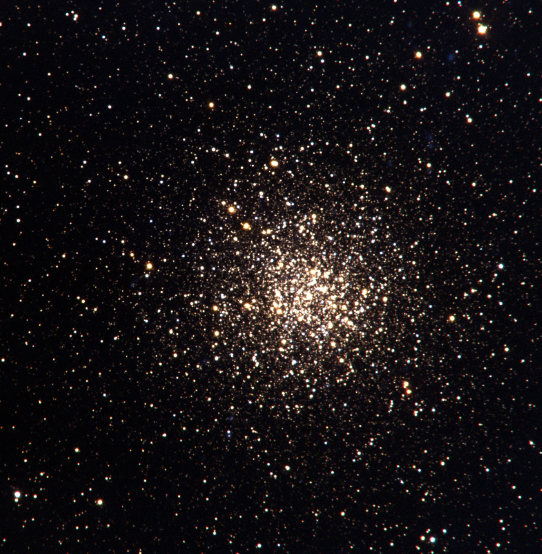
Figure 9 – Old Cluster
(Written by: Mia Mese)
Stellar Colors Connection to Measured Ages
The star clusters we looked at give us a beautiful timeshot of stars around the same age but at different points in their evolution. Essentially, the HR diagrams we produced show how each image resembles the measured ages. A deep analysis of the intrinsic colors reveals various properties of stars, especially their age. An important principle is how as stars age, they run out of hydrogen to burn and decrease the amount of energy they emit. The HR diagram helps us to measure and compare the temperature and luminosity of stars. By knowing the colors or magnitudes of the stars, we convert these into temperature and luminosity measurements. Stars that are more massive are hotter, giving them a blue color, and smaller stars have a lower luminosity and are cooler, giving them a red undertone, In the HR diagram, we were also able to determine the ages of clusters by locating main sequence turnoff points and comparing with models of stellar evolution. Comparing and matching out data to other models of stellar evolution, also known as isochrones, which are curves on the HR diagram, helps us identify and recognize properties of stars/star clusters such as metallicity, reddening, and age.
For instance, red giant stars trace out a horizontal line whereas main sequence stars trace out a diagonal path. Additionally, by allocating and analyzing where exactly the main sequence turnoff is and the distance of the stars not in the main sequence evolved, we can determine the cluster’s age.In the very early stages of a star cluster’s formation, most high mass stars will lie in the main sequence while lower mass stars will be in the T Tauri phase. In the much later stages, almost 10 billion years after, the OBAFG stars will no longer be in the main sequence, with stars in the red giant and white dwarf areas.
Let’s first look at figure 1, IC 2948, which consists of a couple really big and bright blue stars, and a few smaller, reddish orange stars. The HR diagram for IC 2948 is very similar to the isochrone and follows on the black line perfectly. The colors are also very vibrant and luminous, indicating a relatively young cluster. Now let’s look at figure 5, NGC 4349, which consists of an almost balanced mix of small-medium red/orange stars and blue stars. Unlike figure 1, NGC 4349 shows a few more reddish orange stars that are bigger than the blue stars. Moreover, a look at the HR diagrams shows us how the cluster follows the isochrone for the most part, with slight variances and dispersion of the stars throughout. The stars are also very pigmented or bright on the diagrams. Finally, figure 9, NGC 3201, consists of almost entirely red and orange stars, with blue stars less notably sprinkled around the outer radius. A look at the HR diagram also shows how the stars don’t follow the model (isochrone) and are more dispersed throughout compared to the HR diagrams of the previous sections, which are younger. Another important observation is how the colors are also less luminous or bright. Comparing figure 9 and figure 5 shows us how figure 9 contains more dull stars on both ends of the spectrum (red and blue). Analyzing and comparing all 3 figures (1, 5, and 9) side-by-side shows us how the differences in th colors, paths, and dispersion can tell us a lot about the age of a star. The youngest one consists of the brightest stars, following a diagonal main sequence and the oldest one consists of a duller, more dispersed throughout (in a horizontal path) group of stars.
Ultimately, a star’s color gives us a direct measurement of its surface temperature, which in turn tells us important information about its age. The hotter the star, the faster particles inside the star will move, and the more energy they radiate- and vice versa. Class O stars will be the bluest, and also the youngest, no more than a few million years old. Class M stars will be the reddest, and the oldest, and likely a few billion years old. Class M stars are also the most common in our vast cosmos.
(Written by: Saki Male)
Authors of Blog
Saki Male, Nathan Flinchum, Delanie Mitchell, & Mia Mese